normalization – Graeme Potts Portfolio

The first thing any good game programmer needs to understand when creating either 2D or 3D platform games is a basic understanding of linear algebra. The first thing we need to know about linear algebra is how to use vectors. Everything from the complex calculations of rigidbody mechanics to the simple positioning of a button in a graphical interface requires the use of vectors. A vector is a geometric object that is defined as having a direction and a magnitude (or length). How vectors are perceived often depends on whether the vector is a bound vector or a free vector. A bound vector is defined by having an initial point and a terminal point while a free vector has no definite start or end point.

Vectors themselves are generally categorized into two types: position vectors and direction vectors. Position vectors represent a particular point in space. However they are considered a form of bound vector since they can also be visualized as an arrow starting at the origin whose terminal point is its given position in space. Direction vectors are simply a form of free vector, since they generally do not have any one start or end point. Velocity, acceleration and forces are some of the most commonly used direction vectors. Rays are different from either of these types of vectors since they can be considered a kind of semi-bound vectors. That is to say that they have a definite start point and a direction, but no specific end point (See Raycasting). To understand how useful these constructs are, let us look at some of the operations that we can perform on vectors. For the sake of consistency, I will use capital letters to represent position vectors and lowercase letters to represent direction vectors.

Scalar Multiplication of Vectors:
A scalar is simply a one-dimensional vector and is wholly defined by its magnitude. Time is a common example of a scalar value often found in game logic. Often in games we will want to be able to update the position of an object based on its current velocity. To do that we will need to calculate the displacement. We can get this displacement vector easily through scalar multiplication. All we have to do is multiply each of the components of the velocity vector by the scalar value of time. In the following example $\Delta\vec{x}$ is the displacement vector, $\vec{v}$ is the velocity vector, and $t$ is the time elapsed since the last update:

$\Delta\vec{x} = t\vec{v} = t * \begin{pmatrix}v_x \\ v_y\end{pmatrix} = \begin{pmatrix}t * v_x \\ t * v_y\end{pmatrix}$

This property is both commutative, i.e. $t\vec{v} = \vec{v}t$ , and distributive, meaning that:

$s(\vec{u} + \vec{v}) = s\vec{u} + s\vec{v}$ and $(s + t)\vec{u} = s\vec{u} + t\vec{u}$

Vector Addition:

Here we have two vectors $\vec{a}$ and $\vec{b}$ which sum to form a third vector $\vec{c}$ . We see $\vec{c}$ is the vector we obtained when we place the vectors $\vec{a}$ and $\vec{b}$ head to tail and draw a new vector from the free tail to the free head. It also represents the diagonal of the parallelogram formed by $\vec{a}$ and $\vec{b}$ . This is achieved by simply adding the individual components of the first vector to the corresponding components of the second vector. In two dimensions we would get:

$\vec{a} + \vec{b} = \begin{pmatrix}a_x \\ a_y\end{pmatrix} + \begin{pmatrix}b_x \\ b_y\end{pmatrix} = \begin{pmatrix}a_x + b_x \\ a_y + b_y\end{pmatrix} = \begin{pmatrix}c_x \\ c_y\end{pmatrix} = \vec{c}$

where $\vec{a} = (a_x, a_y)$ and $\vec{b} = (b_x, b_y)$ . Vector addition is both commutative and associative. Associative means that:

$(\vec{a} + \vec{b}) + \vec{c} = \vec{a} + (\vec{b} + \vec{c})$ .

This is how we can apply changes in position due to velocity as well as changes in velocity due to acceleration.

Vector Subtraction:
Suppose we have two points $\vec{A}$ and $\vec{B}$ and we want to find the displacement vector $\overrightarrow{AB}$ from a point $\vec{A}$ to point $\vec{B}$ . We can achieve this by simply subtracting the vector components of initial point $\vec{A}$ from the components of the terminal point $\vec{B}$ like so:

$\overrightarrow{AB} = \vec{B} - \vec{A} = \begin{pmatrix}b_x \\ b_y\end{pmatrix} + \begin{pmatrix}a_x \\ a_y\end{pmatrix} = \begin{pmatrix}b_x - a_x \\ b_y - a_y\end{pmatrix}$

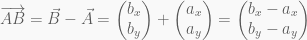
From the picture we see that vector subtraction can be represented as a compound operation of both scalar multiplication and vector addition by negating the first vector (multiplying it by $-1$ ) and taking the sum of $-\vec{A}$ and $\vec{B}$ .

Magnitude:
Sometimes it is important to know how long a vector is along its direction. To do this we simply plug the vector components into the Pythagorean Theorem. I will use the notation $\|\vec{v}\|$ to represent the magnitude or length of a vector $\vec{v}$ with components $v_x$ and $v_y$ . So by the Pythagorean Theorem:

$\|\vec{v}\|^2 = v_x^2 + v_y^2 \implies \|\vec{v}\| = \sqrt{v_x^2 + v_y^2}$

The Pythagorean Theorem also works to find the magnitude of higher dimension vectors as well. For example, in three dimensions we have:

$\|\vec{v}\|^2 = v_x^2 + v_y^2 + v_z^2 \implies \|\vec{v}\| = \sqrt{v_x^2 + v_y^2 + v_z^2}$

This is useful because it gives us the absolute scalar distance between the vector’s initial and terminal point.

Normalization:
When we are dealing with directions, sometimes it is helpful to make sure that they have unit length (a magnitude of exactly one unit of measurement). Suppose we have a unit direction vector and a scalar velocity. To get the velocity as a vector we simply multiply the direction vector by the scalar velocity. But how do we get a normalized vector? Simple, we merely divide each of the vector components by its magnitude. I shall use the notation $\hat{v}$ to denote a normalized vector. So the formula for a normalized vector is simply:

$\hat{v} = \frac{\vec{v}}{\|\vec{v}\|} = \begin{pmatrix}v_x / \sqrt{v_x^2 + v_y^2} \\ v_y / \sqrt{v_x^2 + v_y^2}\end{pmatrix}$

Dot Product:
The dot product is one of the most useful operations in linear algebra and has many practical uses in making video games. It is often called the scalar product because it produces a numerical quantity. The dot product of two vectors $\vec{a}$ and $\vec{b}$ is defined algebraically for three dimensional vectors by the following formula:

$\vec{a} \bullet \vec{b} = a_x b_x + a_y b_y + a_z b_z$

Not very interesting at first, although it is worth mentioning that the dot product of a vector with itself is equivalent to the square of its magnitude. Also note that this property is not only commutative, but also distributive. That is:

$(\vec{a} + \vec{b}) \bullet \vec{c} = \vec{a} \bullet \vec{c} + \vec{b} \bullet \vec{c}$

However, where this formula draws meaning from is its geometric definition. Geometrically the dot product is defined as:

$\vec{a} \bullet \vec{b} = \|\vec{a}\| \|\vec{b}\| \cos{\theta}$

where $\theta$ is the minimum angle between the vectors $\vec{a}$ and $\vec{b}$ . The angle $\theta$ holds significant importance in a variety of situations from vector projection to collision detection. We can calculate the angle quite simply by rearranging the formula to get:

$\theta = \arccos(\frac{\vec{a} \bullet \vec{b}}{\|\vec{a}\| \|\vec{b}\|})$

If $\vec{a}$ and $\vec{b}$ are normalized vectors, this formula simplifies to:

$\theta = \arccos(\hat{a} \bullet \hat{b})$

However, there are many cases where it is not necessary to calculate the angle since the dot product is sufficient. This is convenient to programmers since the dot product is a much cheaper and more efficient operation than say the inverse cosine and anything that saves CPU cycles is a great boon to game programmers.

Cross Product:
The cross product is used in game logic in a variety of ways from game camera projection to quaternions. Since the cross product is most commonly used in terms of three dimensional space I will not cover how the cross product is applied to higher order vectors, despite the fact that their are applications for higher order cross products in game logic and computer graphics. Also keep in mind that all the vector operations covered thus far can be easily expanded to higher dimensions as well but are typically restricted to 2-4 dimensions (4 dimensional vectors are most commonly used in shaders to represent RGBA values).

In general the cross product is a binary operation used to calculate a vector which is orthogonal to each of its input vectors. In the more practical terms of three dimensional space, it takes two vectors $\vec{a}$ and $\vec{b}$ and forms a third vector $\vec{c}$ which is perpendicular to both $\vec{a}$ and $\vec{b}$ and thus normal to the plane that contains $\vec{a}$ and $\vec{b}$ .

An important note to make is that the cross product of two vectors is NOT commutative. The order does matter in determining which direction the resulting vector points. In fact, the vector products $\vec{a} \times \vec{b}$ and $\vec{b} \times \vec{a}$ are related in the following way:

$\vec{a} \times \vec{b} = - \vec{b} \times \vec{a}$

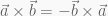
So although they have equal magnitude they point in opposite directions. Additionally, how we actually calculate the cross product of two vectors depends on whether we are using left-handed or right-handed coordinates. It is important to understand this distinction because it depends on which computer graphics API you use as to which coordinate system you should use to write your cross product implementation. DirectX, for example, uses a left-handed coordinate system, whereas OpenGL uses a right-handed coordinate system.

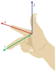
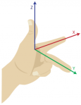
A right-handed coordinate system is simply a three dimensional coordinate system that satisfies the right-hand rule. The right-hand rule states that the orientation of the vectors’ cross product is determined by placing the x-axis and the y-axis tail-to-tail, flattening the right hand, extending it in the direction of the x-axis, and then curling the fingers in the direction that the angle the y-axis makes with the x-axis. The thumb then points in the direction of the z-axis. The left-hand rule simply follows the same procedure but with the left hand (See below).

The cross product in right-handed coordinates is defined as follows:

$\vec{a} \times \vec{b} = \begin{pmatrix} a_y b_z - a_z b_y \\ a_z b_x - a_x b_z \\ a_x b_y - a_y b_x \end{pmatrix}$ (right-handed)

In left-handed coordinates we get:

$\vec{a} \times \vec{b} = \begin{pmatrix} a_z b_y - a_y b_z \\ a_x b_z - a_z b_x \\ a_y b_x - a_x b_y \end{pmatrix}$ (left-handed)

Summary:

With this you should have a basic understanding of vector math and some of the ways it can be applied to video games. In my next post I will cover some more advanced things that can be accomplished with vectors along with some sample code written in C++. Click here for Part 2.

Resources:

Lay, David C. (2005). Linear Algebra and its Applications Third Updated Edition. Addison Wesley. ISBN 978-0-321-28713-4.

External Links:

Linear Algebra for Game Developers

Vector Math