Projects

Here is where I keep a brief list of some of the projects I have worked on so that anyone who visits my blog can quickly view my past and current projects.

The following are my most recent projects:

Character Modeling and Animation in Maya

Cripple Mr. Onion

Captain Polly’s Booty

A* Pathfinder in Unity

Character Modeling and Animation in Maya

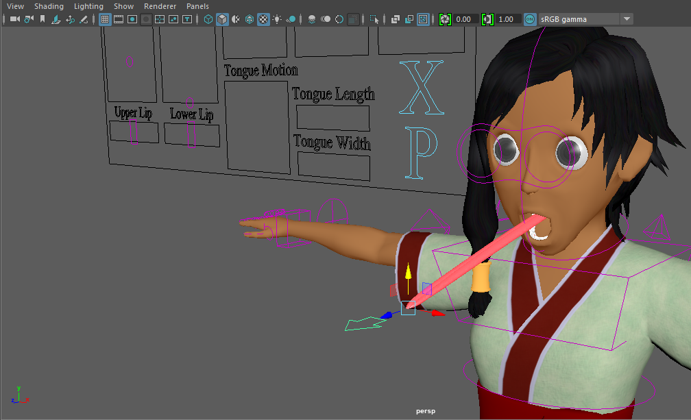
My latest project in game development is to create a fully animated player character designed to be easily portable into a game engine be that Unity, Unreal Engine or someone’s custom made game engine. This is still a work in progress so it is difficult to say when it will be finished, but here is a demo showing the character in its classic T-pose as well as its completed walk animation.

For the remainder of this post I would like to give out some tips to anyone wishing to create similar works in Maya. It may not look like it but this was the first time creating a character model and animation in Maya, which is why I would to give out some tips on how to avoid some of the same beginner mistakes that I made when working on this project.

Getting Started:

The first thing any good modeler needs to get started is some reference material of what they want their character to look like from various angles. For bipedal characters it is generally preferred to model your character starting in the T-pose and to import image planes featuring at least the front and side profiles of your character. This may seem like a high hurdle for those of you who lack artistic talent, but don’t panic because I myself am not artistically inclined either. If you already have a character in mind that someone has already created plenty of reference material for you to use it may not be as difficult as you think to modify the image into a T-pose. The following images are a front and side profile of a character that I created using only Adobe Illustrator’s pen tool and built-in rulers. I based my model on a character that appeared in a manga that I read online called Flower Flower and used various images from that manga as reference material.

You may have noticed that for the side profile I didn’t bother to draw the arm since most of the detail would be lost, not to mention it is not really necessary to model the arm from the side view. You may find that you need additional reference material for finer details such as the hands. When you want to save your reference or texture images to your project folder you want to make sure you save them to your sourceImages folder instead of your images folder since the images folder is where Maya saves its rendered images when doing a batch render. One final thing to note when importing your images into Maya is that many people prefer not to use Maya’s built-in image plane feature because they find it difficult to work with, for example one problem that I frequently had when trying to work with them was that I sometimes found that was unable to select them in the viewport even when I made sure that the layer that they were in was neither a template nor a reference. Eventually I got so annoyed that I replaced them with polygon planes with a transparent file texture.

Modeling:

I will not cover how to do the actual modeling but I can give some suggestions as to where to start. Here are some popular tutorial series that I used to help me model my character:

Maya LT Advanced Training: Character Modeling by Matthew Doyle (recommended)

3D Character Modeling: The Geek by Carol Ashley

One place where the the first tutorial series mentioned above is particularly useful is in described how to best model the head with good topology however it doesn’t really explain why good topology is so important. If you want to learn more on this I suggest watching Modeling a head with proper topology on the Maya Learning Channel. In particular I suggest looking at the third video in the series since it gives a color coded visual representation of how you may want your finished head to look.

One thing I suggest for a character of this nature is to model the body and the clothes as separate objects to start off with. This can be helpful later if you want to be able to model the character in different outfits. In the animation demo above the coat, sash and pants are attached to the body using a simple wrap deformer while the shoes are a part of the main model. Keep in mind that we generally want our game characters to have a range of about 5,000-25,000 tris. My character currently has around 27,000 tris, however I can reduce this number if I delete much of the internal geometry that will be hidden by the clothes. Ideally the pants will be merged with the main body before getting imported into our game engine. The coat and sash may need to dealt with differently depending our game engine since we probably want it to behave in a more realistic fashion.

Texturing:

If like me you are artistically challenged like me many of you may wish to skip making your own custom textures for your character. I only took the time to create my own texture because I wanted to see what it would like textured and although it is plain to see that my textures could use some polishing I am quite proud of the results. However, even if you do not wish to create your own textures you should at least take the time to make sure your UV maps are clean before proceeding to the next steps. The reason for this is that if you decide to duplicate any part of your mesh either for use in another model or for creating blend shapes for the current model then that UV map gets copied as well and it can be a nightmare having to modify the same UV map from scratch. For more on UV mapping see the last video in the series Maya LT Advanced Training: Character Modeling by Matthew Doyle.

For those of you who do want to try your hand at creating textures here are a few useful links that I found helpful:

Creating Textures for Characters in Autodesk Maya by Ryan Bird

How Do I Make Velvet Texture in Photoshop? by David Weedmark

Create a Linen Texture in Photoshop by Howard Pinsky

Adobe Photoshop – Basic Hair Texture Tutorial for IMVU, Second Life, The Sims & More by YouTube user TheRealMrsMVP

Realistic Eye Texture Painting by Krishnamurti Martins Costa

Rigging:

When it comes time to rig your model be sure to create a new scene file and then just import your model into that file. That way if you ever need to make changes to your model you will not break the functionality of your rig. I highly recommend following this tutorial on character rigging: Creating a Character Rig by the Maya Learning Channel.

There are a couple that the above tutorial does does not mention that you should keep in mind. The first is how to properly use to pull vector constraints. If you follow the tutorial exactly you may never run into the problem that I had, but in case you do here is how you can fix it. When you create your pull vector constraint on your IK arm/leg you may find that the model has twisted slightly and no longer matches your FK arm/leg. This can cause some unsightly snapping when switching between IK and FK. The reason for this is that the object that drives the constraint is not on a plane with the joints that the IK handle controls. To get around this problem we could just recreate our joint structure from scratch making sure that there is no unexpected bend in the joints. Alternatively, we can create a triangular plane and snap its corners to the joints controlled by the IK handle, scale the plane out and make its surface live. then we can snap the object diving the pull vector constraint to that plane. Then when you make your pull vector your IK and FK arm/leg should match.

Another thing to keep in mind is that you will need to have additional joint structures for the head and the jaw. While jaw motion may arguably be handled using blend shapes, you must at least have a couple of head joints so that when you skin your rig you have something to paint your head weights to. If you try to paint your head weights to your neckEnd_result_JNT then when you rotate your head control you will have your model’s eyes popping out of their head due to the spline neck’s rotation.

Although I said that jaw motion could be handled using blend shapes, I prefer the method of using joints. Jaw motion is controlled by a control curve set that is set within a bounding bound grouped together with a bunch of other controls for manipulating facial expressions. I also created a joint structure for my characters tongue which is based closely on the joint structure for the spine. I gave the tongue a dual set of controls so that the animator would have the choice of how they want to be able to manipulate the tongue. The blend mode is controlled by an attribute on the IK head control. In auto mode the animator can use a set of controls grouped with the facial expressions to control the position, length and width of the tongue. In manual mode the animator can directly manipulate the position and rotation of the tongueEnd_bind_JNT which in turn affects the squash and stretch of the tongue.

Blend Shapes:

While joints are useful for animating a change between several poses, blend shapes allow us to change the mesh of our model by blending the positions or our mesh’s vertices between one set of positions and another. This is particularly useful for blending between facial expressions.

When using blend shapes it is important to understand that every vertex in the mesh has an index or number associated with it. When using blend shapes maya interpolates between the positions of vertices with matching indices according to the blend weight. So in order for a model and its blend shape to deform properly the indices of their vertices need to line up. If we duplicate a mesh the vertices of the two meshes should match up appropriately. However, if we modify the topology of the duplicate and then create our blend shape then we are likely to result in what many refer to as the spiky-ball-of-death. So it is incredibly important to maintain the same topology between our original mesh and its respective blend shapes.

However, often it is inconvenient to have to duplicate an entire mesh for each blend shape, especially if all we want to blend is the head. One way we can accomplish this is by separating the part of the mesh that we want to blend from the original mesh and creating our blend shapes from duplicates of this mesh. (I personally like to export this duplicated mesh into a separate file and create my blend shapes there since as Maya scene files grow larger and larger they use up a lot of memory and can slow your system down considerably.) When we want to recombine our separated head to the body mesh simply make sure that you select the mesh that you wish to attach a blend shape to before you select the main body. This ensure that the indices of the vertices that are being blended stay the same. Then when you go to create your blend shape node simply make sure that the option Check Topology is turned off.

Another problem that might crop up when creating blend shapes is the possibility that you may wish to mirror a blend shape. Unfortunately, Maya does not provide any built-in tools that make this easy to accomplish. But fear not, because there is an open source MEL script that can help you accomplish this with little to no effort. It and a video tutorial on how to use it can be found at http://www.animationmethods.com/scripts.

Finally if it turns out that you absolutely need to make changes to your topology there is a way to do it without having to recreate all your blend shapes from scratch. There is a tool called Bake Topology to Targets which (possibly) can give you the results you need. The YouTube video Maya BlendShape Tips and Tricks by Steven Roselle shows how this can be done.

Animation:

Before starting to create our animations it is a good idea to study up on how to use the Maya Trax Editor. The YouTube video Maya Trax Editor Tutorial – by Matty Mac gives a pretty good explanation of how it works. The basic premise is that first we need to create a character set of all the controls that we are going to need within the file that contains our rig. Then starting in a new file we create a reference to our character rig file. Making sure our character set is not selected we key in our animation to the time slider. Next we select our character set, add it to the Trax Editor and then go to Create->Animation Clip->Options and make sure to select the TimeSlider as the source. Then it is a simple task to export the animation clip to your clips folder.

For more advanced animation you can also check out the YouTube video on Animation Layers titled CGI 3D Tutorial HD: “Using Animation Layers in Maya” – by 3dmotive.

Additional References:

Facial Rigging Tutorial by Adam Bailey

Tips and Tricks: Blendshape Heads by Jennifer Conley

Operator Overloading in C++

One of the advantages of working with C++ is the ability of the programmer to overload not only functions, but also operators as well. With operator overloading most operators can be extended to work not only with built-in types like floats and ints but also classes. This gives the programmer the freedom to change how a built-in operator is used on objects of that particular class. For example, we can overload the plus, minus and star operators to perform vector addition, subtraction and scalar multiplication on the components of our Vector3 class. (I will be using this Vector3 class as an example of operator overloading for the remainder of this post. For more on vector math see Vectors Part 1.)

The following code sample is an example of a three dimensional vector class which uses operator overloading for many the the various operators that are available. We will examine the syntax of each of these operators individually.

class Vector3 {
public:
    float x;
    float y;
    float z;

    //Constructor method
    Vector3(float x, float y, float z) : x(x), y(y), z(z) {}

    //unary operations
    Vector3 operator- () const { return Vector3(-x, -y, -z); }

    //binary operations
    Vector3 operator- (const Vector3& rhs) const {
        return Vector3(x - rhs.x, y - rhs.y, z - rhs.z);
    }
    Vector3 operator+ (const Vector3& rhs) const {
        return Vector3(x + rhs.x, y + rhs.y, z + rhs.z);
    }
    Vector3 operator* (const float& rhs) const {
        return Vector3(x * rhs, y * rhs, z * rhs);
    }
    friend Vector3 operator* (const float& lhs, const Vector3& rhs) {
        return rhs * lhs;
    }
    Vector3 operator/ (const float& rhs) const {
        return Vector3(x / rhs, y / rhs, z / rhs);
    }
    bool operator!= (const Vector3& rhs) const {
        return (*this - rhs).sqrMagnitude() >= 1.0e-6;
    }
    bool operator== (const Vector3& rhs) const {
        return (*this - rhs).sqrMagnitude() < 1.0e-6;
    }

    //assignment operation
    Vector3& operator= (const Vector3& rhs)  {
        //Check for self-assignment
        if (this == &rhs)
            return *this;
        x = rhs.x;
        y = rhs.y;
        z = rhs.z;
        return *this;
    }

    //compound assignment operations
    Vector3& operator+= (const Vector3& rhs) {
        x += rhs.x;
        y += rhs.y;
        z += rhs.z;
        return *this;
    }
    Vector3& operator-= (const Vector3& rhs) {
        x -= rhs.x;
        y -= rhs.y;
        z -= rhs.z;
        return *this;
    }
    Vector3& operator*= (const float& rhs) {
        x *= rhs;
        y *= rhs;
        z *= rhs;
        return *this;
    }
    Vector3& operator/= (const float& rhs) {
        x /= rhs;
        y /= rhs;
        z /= rhs;
        return *this;
    }

    //subscript operation
    float& operator[] (const int& i) {
        if (i < 0 || i > 2) throw std::out_of_range("Out of Vector3 range\n");
        return (i == 0) ? x : (i == 1) ? y : z;
    }
    const float& operator[] (const int& i) const {
        if (i < 0 || i > 2) throw std::out_of_range("Out of Vector3 range\n");
        return (i == 0) ? x : (i == 1) ? y : z;
    }

    //typecast operations
    operator Vector2() { return Vector2(x, y); }
    operator Vector4() { return Vector4(x, y, z, 0.0f); }

    ...

};

Unary Operators:

First let us take a look at the negate (-) operator. The body of this operator simply returns a new Vector3 object with each of its floating point components negated. But what we are most interested in is its declaration. Like a typical function it has a return type which is Vector3 and a parameter list enclosed by parenthesis. But instead of a function name we follow the return type with the keyword operator and then the symbol for the particular operator that we wish to overload, which in this case is the minus sign.

Vector3 operator- () const { return Vector3(-x, -y, -z); }

Overloaded operators can be defined either as class member functions or as non-member functions. Here we define them as class member functions. This means that we do not have to include one of the objects involved in the operation in the parameter list since we can reference that object through the this operator (we could have just as easily written the x parameter in the body of the function as this->x). The parameter list for our unary operator is empty because we are only operating on the current object. If we were to write this as a non-member function its declaration would look something like this:

Vector3 operator- (const Vector3& a) { return Vector3(-a.x, -a.y, -a.z); }

Note that the const written after the parameter list in the class member function simply ensures that the function cannot make changes to the original object. The same functionality is accomplished by the presence of the const keyword in the parameter list of the non-member function. If you do wish the operator to make changes to the original object then you would simply remove the const in either of these places.

Binary/Comparison Operators:

Next let us observe the binary operations of addition and subtraction.

Vector3 operator- (const Vector3& rhs) const {
    return Vector3(x - rhs.x, y - rhs.y, z - rhs.z);
}
Vector3 operator+ (const Vector3& rhs) const {
    return Vector3(x + rhs.x, y + rhs.y, z + rhs.z);
}

As you can see their declarations are hardly any different from the unary operator except that they have an additional parameter which we have named rhs to indicate that it is the object that appears on the right-hand side of the operator. Note that the parameter is passed as a constant reference. We already discussed what purpose the const holds in this context, but why pass as reference? Often when we pass an object by reference it is because we want to be able to make changes to the object within the body of the function, but in this case we pass it as constant to prevent that from happening. So why do we do this? The answer is simple. Passing an object by value means that we have to take extra time to make a copy of the object that is passed. Passing by reference allows us to skip that step by simply passing the address of the object, thus making our code more efficient. Comparison operators generally work the same way with the exception that they simply return a boolean value.

Now let us take a look at our multiplication operator.

Vector3 operator* (const float& rhs) const {
    return Vector3(x * rhs, y * rhs, z * rhs);
}
friend Vector3 operator* (const float& lhs, const Vector3& rhs) {
    return rhs * lhs;
}

The first thing we notice is that we actually have two multiplication operator functions. The first one looks just like our addition/subtraction operator declarations except that the parameter is of type float. The second one on the other hand is actually a non-member function that we declare to be a friend of the Vector3 class to ensure that it has access to the Vector3 class’ private methods and variables. Although this class does not have any private methods or variables we still need to declare this function as a friend because otherwise the compiler expects the function to have only one parameter. But why do we need both of these functions in the first place? Strictly speaking, we don’t need both unless we wish to ensure that scalar multiplication is a commutative property of our Vector3 class. Our first function does a scalar multiplication operation for the case where we have a Vector3 object on the left and a scalar (float) on the right of our operator but would not work if we were to reverse the order. That is why we need the second function to perform the operation when the order is reversed. Note that we did not need to do the same thing for the addition operator despite it also being commutative because both the left and the right hand sides are of type Vector3.

Assignment Operators:

Next we will see how we can override the assignment operator.

Vector3& operator= (const Vector3& rhs)  {
        //Check for self-assignment
        if (this == &rhs)
            return *this;
        x = rhs.x;
        y = rhs.y;
        z = rhs.z;
        return *this;
    }

Most of the time we do not really need to override the assignment operator because the compiler generated constructor and assignment operator are usually sufficient. But if our class contains pointers the default assignment operator can sometimes lead to problems because we end up with objects that have pointers to the same location. To avoid these problems you will want to know how to override the assignment operator so that it makes a deep copy as well as how to make a copy constructor. I will not be covering how to do either of these things in this post. The example that I give here has no practical purpose since the default assignment operator does exactly the same thing. However, there are two things worth mentioning if you ever do decide to overload the assignment operator. The first is that, if you want your class to support chain assignment (see example below), the function should return the address of the current object. The second is that you should always check for self-assignment before altering any data otherwise your class may end up releasing the resources that it is trying to copy from.

Compound assignment operators are generally simpler to understand. They combine normal binary operations with an assignment operator.

Vector3& operator+= (const Vector3& rhs) {
    x += rhs.x;
    y += rhs.y;
    z += rhs.z;
    return *this;
}

Unlike normal binary operators they are generally meant to make changes to the original object, but like the assignment operator they usually return the address of the object. This allows the programmer to write statements like the following:

a = b += c -= d *= e;  //example of chain assignment

Subscript/Function Call Operators:

Next we have the subscript operator.

float& operator[] (const int& i) {
    if (i < 0 || i > 2) throw std::out_of_range("Out of Vector3 range\n");
    return (i == 0) ? x : (i == 1) ? y : z;
}
const float& operator[] (const int& i) const {
    if (i < 0 || i > 2) throw std::out_of_range("Out of Vector3 range\n");
    return (i == 0) ? x : (i == 1) ? y : z;
}

Here I define it so that the subscript operator returns one of the vector components based on the integer value passed. Notice however that once again we have two functions. The first behaves just as we would expect. The second one on the other hand is written as a constant function that returns a constant reference. Here the const at the end of the second member function allows the function to be called even on an object that is defined as constant. Without this function the programmer would not be able to access the contents of a constant object using the subscript notation. The reason we return a constant reference is to ensure that the caller cannot modify the contents of our constant vector object.

If we were overloading the function call operator we would similarly wish to define two functions, one for constant objects and one for non-constant objects. We do not override the function call operator in the Vector3 class, but something to keep in mind is that, unlike other operators, the function call operator can have as many parameters as the programmer likes. An example where this might be useful is in a matrix class where the programmer wishes to look up a matrix element by its row and column. You cannot do this with the subscript operator because it only takes one parameter, but it can be done in the following way:

class Matrix4x4 {
private:
    float data[16];
public:
    float& operator() (const int& row, const int& col) {
        return data[row + (col * 4)];
    }
    const float& operator() (const int& row, const int& col) const {
        return data[row + (col * 4)];
    }

    ...
};

Typecast Operators:

Operator overloading can even be used to define typecasting operations for our user-defined classes. Suppose elsewhere we have defined a two-dimensional and a four-dimensional vector class and we want our compiler to know how to cast our Vector3 object into one of these types. We can accomplish this in the following way:

operator Vector2() { return Vector2(x, y); }
operator Vector4() { return Vector4(x, y, z, 0.0f); }

Here we simply write the operator keyword followed by the type we want to cast our object into followed by open and close parentheses. We do not need to define a return type since C++ assumes that we will return the correct type. With the help of these functions we should be able write lines of code like the following without our compiler spitting out an error:

Vector2 v2 = Vector2(1.0f, 2.0f);
Vector3 v3 = Vector3(3.0f, 4.0f, 5.0f);
Vector4 v4 = Vector4(6.0f, 7.0f, 8.0f, 9.0f);
v2 = v3; //compiler implicitly typecasts to Vector2
v4 = v3; //compiler implicitly typecasts to Vector3

End of Lesson:

Well that is it for my lesson on operator overloading. I hope the things you have learned here will be of use to you in designing your C++ applications. If you are interested in reading some more of my postings, you may follow the links below:

Sprite Animation in Java

In this posting I will be describing the process by which we can program a simple sprite-based animation. A sprite is simply a two-dimensional graphical image that is integrated into a larger scene. They are a popular tool for populating scenes in video games as they are easily manipulated separately from the rest of the scene. To animate it we need a series of image frames for each individual sprite. These are often stored collectively in a single image called a spritesheet. When we draw our sprite we only draw one frame at a time. Then as time passes we just switch between our frames to give the illusion that our sprite is moving. I will be writing the sample code for this example in Java, but it should not be too hard to adapt it to other languages.

The first thing we want to do is define a structure to store each frame of our animation. The purpose of this is to put some separation between the constant definitions that are shared between animations of a single type and the constantly updating data of the individual animation objects. In it we will store three things: the image associated with this frame, the number of the frame indicating where in the list of frames it belongs, and the duration of time that the animation should spend on this one frame.

// AnimationFrame.java
import java.awt.image.BufferedImage;
public class AnimationFrame {
    public final BufferedImage image;
    public final int frameNumber;
    public final int duration;

    public AnimationFrame(BufferedImage image, int frameNumber, int duration) {
        this.image = image;
        this.frameNumber = frameNumber;
        this.duration = duration;
    }
}

Next we can create our Animation class. In it we store a list frames in the order that they should be played, the name of the current animation, the index of the current frame, the amount of time that needs to elapse before we switch to the next frame and a boolean variable to indicate whether or not the animation is currently playing. Optionally we can also include a boolean variable to allow the animation to loop back the the beginning once the final frame has been shown.

Most of the work done by the Animation object is done within our update method which is meant to be called every frame before we draw our Sprite to the screen. It takes as a parameter the amount of time that has elapsed since our last update. We subtract this time from our timeToNext value and if the result is negative we know that it is time to switch to the next frame. then we increment our timeToNext variable by the duration of the next frame. The rest is just a matter of providing methods that allow the client to start, stop and pause the animation. If you are a fan of the Observer Pattern you can even include a custom listener class object whose functions are called when certain state changes are made within the Animation class. We could make such an interface in just a few lines like so:

// AnimationListener.java
public interface AnimationListener {
    public void onComplete(); // gets called when animation reaches end (unless looping)
    public void onStart();    // gets called when the animation's start method is called
    public void onPlay();     // gets called when the animation's play method is called
    public void onPause();    // gets called when the animation's pause method is called
    public void onStop();     // gets called when the animation's stop method is called
}

One final note to make is that if you wish your program to be multithreaded, it may be a good idea to define any function calls that alter your animation’s state using the synchronized keyword.

// AnimationClip.java
import java.awt.image.BufferedImage;
import java.util.ArrayList;
import java.util.List;

public class AnimationClip {
    private final List<AnimationFrame> frames;
    private final List<AnimationListener> listeners;
    private String name;
    private int timeToNextFrame;
    private int currentFrame;
    private boolean playing;
    private final boolean loop;

    /**
     * Class constructor
     * @param name name of the clip
     * @param frames ordered list of frames
     * @param loop boolean value determining whether the clip should repeat itself
     */
    public AnimationClip(String name, ArrayList<AnimationFrame> frames, boolean loop) {
        this.frames = frames;
        this.name = name;
        this.loop = loop;
        listeners = new ArrayList<>();
        playing = false;
        currentFrame = 0;
        timeToNextFrame = (frames.size() > 0)? frames.get(currentFrame).duration : 0;
    }

    /**
     * Gets the name of the clip
     * @return the name
     */
    public String getName() {
        return name;
    }

    /**
     * Gets whether the clip is playing
     * @return true if clip is currently playing
     */
    public boolean isPlaying() {
        return playing;
    }

    /**
     * Gets the current frame of the animation
     * @return the frame image or null if there are no frames
     */
    public synchronized BufferedImage getFrame() {
        return (frames.size() > 0)? frames.get(currentFrame).image : null;
    }

    /**
     * Starts the clip from the beginning
     */
    public synchronized void start() {
        playing = true;
        currentFrame = 0;
        timeToNextFrame = (frames.size() > 0)? frames.get(currentFrame).duration : 0;
        for (AnimationListener listener : listeners) listener.onStart();
    }

    /**
     * Starts the clip from the current frame
     */
    public synchronized void play() {
        playing = true;
        for (AnimationListener listener : listeners) listener.onPlay();
    }

    /**
     * Pauses the clip
     */
    public synchronized void pause() {
        playing = false;
        for (AnimationListener listener : listeners) listener.onPause();
    }

    /**
     * Stops the clip and sets the current frame back to the beginning
     */
    public synchronized void stop() {
        playing = false;
        currentFrame = 0;
        timeToNextFrame = (frames.size() > 0)? frames.get(currentFrame).duration : 0;
        for (AnimationListener listener : listeners) listener.onStop();
    }

    /**
     * Updates the animation based on the amount of time that has elapsed.
     * Note: Will only update if the animation is currently playing
     * @param elapsed
     */
    public synchronized void update(long elapsed) {
        if (!playing) return;
        timeToNextFrame -= elapsed;
        if (timeToNextFrame < 0) {
            int numFrames = frames.size();
            ++currentFrame;
            if (currentFrame >= numFrames) {
                if (loop) currentFrame = 0;
                else {
                    // end of the animation, stop it
                    currentFrame = numFrames - 1;
                    timeToNextFrame = 0;
                    playing = false;
                    for (AnimationListener listener : listeners)
                        listener.onComplete();
                    return;
                }
            }
            AnimationFrame current = frames.get(currentFrame);
            timeToNextFrame += current.duration;
        }
    }

    /**
     * Adds a listener to the list of listeners
     * @param listener the listener to add
     */
    public void addAnimationListener(AnimationListener listener) {
        listeners.add(listener);
    }
}

Game Programming: Math Libraries

Most game engines define their own custom set of math libraries for use in their games. Unity, for example, has defined its own Mathf library for performing common operations on floating point numbers. You may wonder what is wrong with just using System.Math as apposed to UnityEngine.Mathf. Some people use Mathf instead of Math because it saves them the trouble of having to do double to float conversions. However, in most cases Math is considered faster than Mathf. Standard math libraries are certainly convenient and will most often be more efficient than any math libraries that you roll yourself, so why go to the trouble of implementing a custom library. The problem with standard math libraries is that they may not always have the kinds of functions that are most important to game programming. Other times it may be better to forgo accuracy in favor of efficiency by replacing expensive operations such as cos, sin and e^x with less expensive and less accurate approximations of these functions. In this article I will discuss some of the most commonly used functions found in Unity’s Mathf library and how you may implement them yourself.

Approximately:

Due to the nature of floating point numbers it is very common for operations performed on them to result in some form of rounding error. This can lead to problems when trying to compare the equality of floating point numbers. For example we may end up comparing a number like 2.0 to a number like 1.999999999. For all effects and purposes these numbers are practically the same but when we check for equality we get a false statement. This is why we sometimes need to take into account some margin of error when comparing floats. This is exactly what the Mathf.Approximately function does. It can be implemented in the following way:

bool Approximately(float a, float b) {
    return Abs(a - b) < Epsilon;
}

Here we take the absolute value of the difference between the two input variables and check if it is less than some arbitrarily small value called Epsilon. It should be noted however that although some standard math already have a predefined value for epsilon, it may actually be better for the programmer to define their own value for epsilon since the standard math library’s definition of epsilon may be too small to make any difference from straight equality comparison. An alternative approach could also be to define an Approximately function that takes the tolerance as a parameter and just replace Epsilon with this tolerance value.

Clamp:

Clamp is such a useful tool that it is any wonder why it is not a common tool found in every math library, especially since it is so simple to write. Perhaps it is just so simple that some programmers feel it is not necessary to include it in a standard math library. Simply put, clamp ensures that its input value lies within a certain range of values. If the number lies between the given range it simply returns the number itself, otherwise it returns the nearest endpoint. An example where this might be useful is in the case where the programmer wants to ensure that a player character never goes past the edges of the screen. All the programmer has to do is Clamp the player’s position to within the screen boundaries. Clamp can be implemented in the following way:

float Clamp(float value, float min, float max) {
    return (value < min)? min : (value > max)? max : value;
}

This function is so useful that Unity has even included a Clamp01 function that specifically clamps a floating point value to between 0 and 1.

Linear Interpolation (Lerp):

Linear interpolation is the process by which we find a point somewhere between two input values. We can visualize it as a line drawn between two points. Using the equation for a line we can write the formula for the desired value $y$ as $y = a + (b - a)x$ where $a$ and $b$ are the start and end values respectively and $x$ represents what fraction of the way we are between our two values. Note that we only get a value between $a$ and $b$ when $x$ lies within the range $[0, 1]$ ; any other value for $x$ results in some value outside the interval $[a, b]$ . We also see that $y = a$ when $x = 0$ and $y = b$ when $x = 1$ . However, to avoid rounding error caused by floating point arithmetic, it is best to rewrite the equation as $y = a(1 - x) + bx$ (this ensures that $y = b$ when $x = 1$ ). Depending on how you want your Lerp function to behave for certain values of $x$ you may wish to clamp it to between $0$ and $1$ so as to never overshoot the endpoints. However, in some rare cases it may be better to leave the value unclamped. The following code sample shows how we may implement the former:

float Lerp(float a, float b, float t) {
    t = Clamp01(t);
    return a * (1 - t) + b * t;
}

For more help learning the proper use of linear interpolation, see How to Lerp like a Pro by Robert Utter.

Move Towards:

While linear interpolation certainly has its uses, it is sometimes not entirely practical since it requires the programmer to know what point we started at and what fraction of the way between the two points we are at a given time. But suppose instead we want to procedurally step some value towards some target using some kind of displacement value. We want a way to find our new value while making sure that we do not overshoot our target. To do this we simply compare our expected displacement to the difference between our current value and our target value. If our expected displacement is greater than the actual distance to our target then we just return our target value. Here is an example:

float MoveTowards(float current, float target, float maxDelta) {
    float delta = target - current;
    return (maxDelta >= delta) ? target : current + maxDelta;
}

Note that in the implementation above a negative value of maxDelta will cause our output to procedurally step away from our target value.

Smooth Damp:

While MoveTowards generally serves its intended purpose it can often result in game mechanics that look somewhat jerky since it forces something to come to a sudden stop once it reaches its goal. If we want our game to look somewhat cleaner we need to apply smoothing to our calculations. One way that we can apply smoothing is to apply some kind of S-curve to give us that smooth ease-in/ease-out motion. One commonly used formula is $x = 6t^5 - 15t^4 + 10t^3$ which gives us such an S-curve and can be used with little computing cost.

Another technique to achieve smoothing is through exponential decay. This is a kind of ease-out method of smoothing and can be accomplished by the statement $x = x + (desiredX - x) * 0.1f * timeDelta$ where $timeDelta$ is the time step between updates. The advantage of this type of smoothing is that you can smooth toward a changing target and you do not need to know how much time has elapsed since the start. However, the problem with this type of smoothing is that the initial motion is sudden.

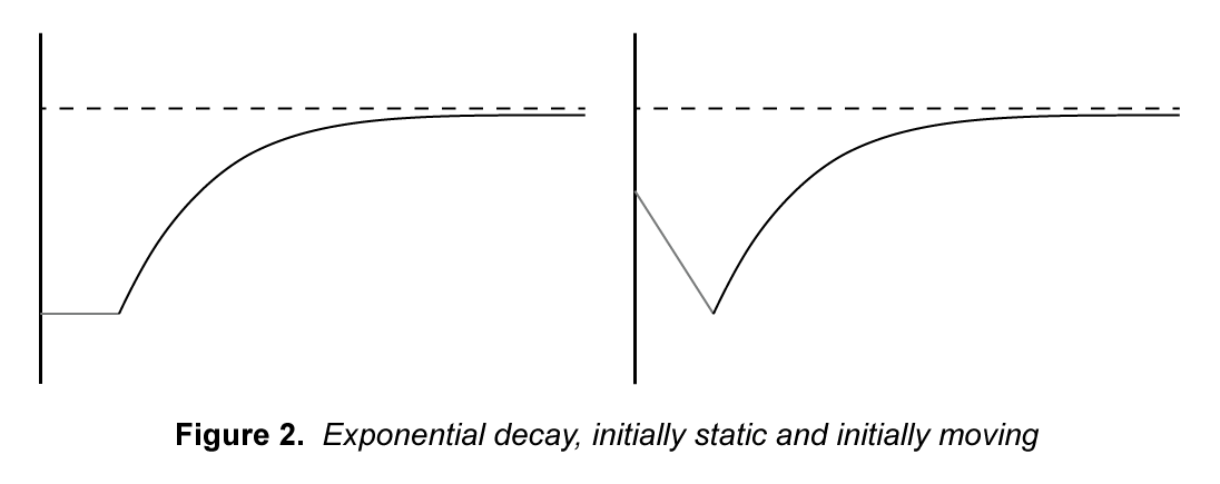
The approach we will be using, however, will rely on the model for a critically damped spring. This model fixes the problem we have with the exponential decay model by maintaining the ease-in property found in the S-curve.

A spring will always try to maintain a certain length by exerting a force that pushes it towards that desired length. Without damping this system will oscillate back and forth past the desired length forever. We say the system is critically damped when it returns to equilibrium in the least possible amount of time. We can write the equation for the force acted on the spring as $F = -k(x - x_d) - bv$ where $k$ is the spring constant, $x_d - x$ is the displacement from our desired position, $b$ is the damping coefficient and $v$ is the velocity of the end of the spring that works to slow the spring down. Using Newton’s second law of motion, $F = ma$ , and writing the velocity and acceleration as the first and second derivatives of the position, we can obtain the ordinary differential equation (ODE):

$m\frac{d^2x}{dt^2} + b\frac{dx}{dt} + kx = kx_d$ (1)

The next step requires us to know how to solve for an equation of $x$ . The above ODE will have a solution of the form $x(t) = x_p(t) + x_c(t)$ where $x_p(t)$ is a particular solution of the equation and $x_c(t)$ is the complementary solution of the associated homogeneous DE. We see that the particular solution is of the form $x_p(t) = A$ where $A$ is a constant since the right side of Equation 1 is constant. By taking the first and second derivatives of $x_p(t)$ and plugging them into Equation 1 we see that $A = x_d$ .

That was our particular solution; now let us find our complementary solution. The homogeneous DE gives us the characteristic equation $mr^2 + br + k = 0$ which has the roots:

$r = \frac{-b \pm \sqrt{b^2 - 4mk}}{2m}$

It can be shown that the system will be critically damped when our equation has the real repeated roots $r = -\sqrt{\frac{k}{m}}$ which only occurs when $b^2 = 4mk$ . We can use this to simplify Equation 1:

$\frac{d^2x}{dt^2} + 2\omega\frac{dx}{dt} + \omega^2(x_d - x) = 0$ where $\omega = \sqrt{\frac{k}{m}}$ (2)

In the above formula $\omega$ is the spring’s natural frequency and represents the stiffness or strength of the spring. But now we also have our complementary solution which is $x_c(t) = (c_0 + c_1t)e^{-\omega t}$ . So our general solution is:

$x(t) = x_d + (c_0 + c_1t)e^{-\omega t}$

Solving for the constants $c_0$ and $c_1$ using the initial conditions $x(0) = x_0$ and $x'(0) = v_0$ gives us the actual solution:

$x(t) = x_d + ((x_0 - x_d) + (v_0 + \omega(x_0 - x_d))t)e^{-\omega t}$ (3)

This formula now tells us everything we need to calculate the new position and by taking the derivative we can find the new velocity of the object after after this time step:

$v(t) = (v_0 - (v_0 + \omega(x_0 - x_d))\omega t)e^{-\omega t}$ (4)

Now the only parameters we need for our smoothing function are our current position and velocity, our target position our elapsed time and finally our smoothness factor $\omega$ . But how do we figure out what we should use for our smoothness factor? It would be much more intuitive to control our function based on how long we want it to take to reach equilibrium. If we define this smooth time as being the expected time to reach the target when at maximum velocity, then we solve for it quite simply by setting the acceleration to zero and the maximum velocity to $\frac{x_d - x_0}{t_{sm}}$ where $t_{sm}$ is the smooth time and plugging these values into Equation 2. We then see that $\omega = \frac{2}{t_{sm}}$ .

One final note before we write our smoothing function is that Equation 3 and 4 contain $e^x$ . We talked before about how operations such as these are expensive so the following code shows a polynomial that can be used to approximate $e^x$ . While I do not know exactly how this polynomial is produced, I would hazard a guess and say that it is probably constructed by approximating a higher order Taylor series polynomial down to a third order polynomial. Finally to make our function exactly like the SmoothDamp function of Unity’s Math library we also need to clamp the speed according to some defined max speed.

float SmoothDamp(float current, float target, float& currentVelocity, float smoothTime,
        float maxSpeed = Infinity, float deltaTime = Time.deltaTime) {
    smoothTime = Max(0.0001f, smoothTime);
    float omega = 2.0f / smoothTime;
    float x = omega * deltaTime;
    float exp = 1.0f / (1.0f + x + 0.48 * x * x + 0.235 * x * x * x);
    float deltaX = target - current;
    float maxDelta = maxSpeed * smoothTime;

    // ensure we do not exceed our max speed
    deltaX = Clamp(deltaX, -maxDelta, maxDelta);
    float temp = (currentVelocity + omega * deltaX) * deltaTime;
    float result = current - deltaX + (deltaX + temp) * exp;
    currentVelocity = (currentVelocity - omega * temp) * exp;

    // ensure that we do not overshoot our target
    if (target - current > 0.0f == result > target) {
        result = target;
        currentVelocity = 0.0f;
    }
    return result;
}

Resources:

Kirmse, Andrew. (2004). Game Programming Gems 4. Charles River Media. ISBN 9781-58450-295-1.

Zill, Dennis G. (2009). A First Course in Differential Equations with Modeling Applications. Brooks Cole. ISBN 978-0-495-10824-5

External Links:

Critically Damped Spring Smoothing

How to Lerp like a Pro

Unity Scripting API: Mathf

Unity Forum: Formula behind SmoothDamp

Vectors Part 2: Programming in C++

In my last post I covered the basics of vector arithmetic. In it I wrote about vector addition, subtraction, scalar multiplication, magnitude, normalization, dot products and cross products. This time will we be learning about some more advanced uses of vectors in game programming. Some of these operations you may recognize as methods of the Vector3 class of the Unity Game Engine. Here I will be explaining how you may implement some of these methods for yourself.

I will be presenting the sample code in C++. I chose this language largely because it supports the concept of operator overloading. It is possible to adapt the code to be written in languages like Java by creating free or static member functions for operations like addition, subtraction and scalar multiplication. But if you wish to know more about operator overloading in C++, you may visit my blog post on Operator Overloading.

Projection:

When we have two vectors $\vec{a}$ and $\vec{b}$ we can visualize the first vector $\vec{a}$ as the sum of two vectors $\vec{a}_1$ and $\vec{a}_2$ where $\vec{a}_1$ is the vector component of $\vec{a}$ parallel to vector $\vec{b}$ and $\vec{a}_2$ is vector component of $\vec{a}$ orthogonal to vector $\vec{b}$ . Because $\vec{a}_1$ is in the same (or opposite) direction as $\vec{b}$ it is called the vector projection of $\vec{a}$ onto $\vec{b}$ or $proj_{\vec{b}}\vec{a}$ and its magnitude is called the scalar projection of $\vec{a}$ onto $\vec{b}$ or $comp_{\vec{b}}\vec{a}$ . Similarly $\vec{a}_2$ is called the vector rejection of $\vec{a}$ from $\vec{b}$ .

Sometimes in video games it is necessary to calculate one of these component vectors. Fortunately, since $\vec{a} = \vec{a}_1 + \vec{a}_2$ we can easily calculate $\vec{a}_2$ in terms of $\vec{a}_1$ . So we just need to find $\vec{a}_1$ . We can find the length of $\vec{a}_1$ using the definition of $\cos{\theta}$ where $\theta$ is the angle between $\vec{a}$ and $\vec{b}$ . We know that $\cos{\theta}$ is adjacent over hypotenuse. So we have:

$\cos{\theta} = \frac{\|\vec{a}_1\|}{\|\vec{a}\|} \implies comp_{\vec{b}}\vec{a} = \|\vec{a}_1\| = \|\vec{a}\|\cos{\theta}$

If we recall the geometric definition of the dot product we can simplify this equation to:

$comp_{\vec{b}}\vec{a} = \|\vec{a}\| \|\hat{b}\|\cos{\theta} = \vec{a} \bullet \hat{b} = \frac{\vec{a} \bullet \vec{b}}{\|\vec{b}\|}$

Now that we have its magnitude we can find $\vec{a}_1$ by multiplying this by the unit vector in the direction of $\vec{b}$ . So we get:

$proj_{\vec{b}}\vec{a} = \vec{a}_1 = \|\vec{a}_1\|\hat{b} = (\frac{\vec{a} \bullet \vec{b}}{\|\vec{b}\|})(\frac{\vec{b}}{\|\vec{b}\|}) = \frac{\vec{a} \bullet \vec{b}}{\|\vec{b}\|^2}\vec{b} = \frac{\vec{a} \bullet \vec{b}}{\vec{b} \bullet \vec{b}}\vec{b}$

Reflection:

Now that we know how to calculate the vector projection, we can now calculate the reflection of a vector. This is useful in computer graphics for creating mirror effects. To calculate the reflection of a vector we need only the vector $\vec{v}$ that we are reflecting and the normal $\hat{n}$ of the surface that our vector is reflecting off. For simplicity we will assume that the normal vector is normalized.

We can see by the diagram that $proj_{\hat{n}}\vec{r}$ is the same as $proj_{\hat{n}}-\vec{v}$ . Similarly, the projection of $\vec{r}$ onto the plane whose normal is $\hat{n}$ is the same as the projection of $\vec{v}$ off the plane. This projection can be found by simply subtracting $proj_{\hat{n}}\vec{v}$ from $\vec{v}$ . So by summing the components together we get:

$\vec{r} = proj_{\hat{n}}-\vec{v} + (\vec{v} - proj_{\hat{n}}\vec{v}) = (-\vec{v} \bullet \hat{n})\hat{n} + \vec{v} - (\vec{v} \bullet \hat{n})\hat{n} = \vec{v} - 2(\vec{v} \bullet \hat{n})\hat{n}$

Orthonormalization:

To understand the process of orthonormalization, we first need to understand the concept of vector spaces and bases. A vector space $V$ is quite simply a set, whose elements are vectors, for which we have defined two operations: vector addition and scalar multiplication. One example of $V$ would be the n-dimensional Euclidean space $\mathbb{R}^n$ . For the following operation we will be looking specifically at $\mathbb{R}^3$ . A basis of a vector space is a subset of vectors $\vec{v}_1, \dots, \vec{v}_n$ in $V$ which span the vector space and are linearly independent, that is $\vec{v}_i \neq k\vec{v}_j$ for any scalar constant $k$ when $i \neq j$ . We say that a basis spans a vector space so long as any vector $\vec{v}$ in the vector space can be uniquely written as:

$\vec{v} = a_1\vec{v}_1 + a_2\vec{v}_2 + \dots + a_n\vec{v}_n$

for some set of scalar values $a_1, a_2, \dots , a_n$ . An orthonormal basis is simply a basis whose vectors are normalized and whose inner product is $\langle \vec{v}_i, \vec{v}_j \rangle = 0$ when $i \neq j$ . The inner product is just a generalization of the dot product as it is applied to a set of vectors. So what $\langle \vec{v}_i, \vec{v}_j \rangle = 0$ means is that all the vectors in the set are mutually orthogonal to one another. For example the standard basis of the Cartesian coordinate system defines a point in 3D space by:

$\vec{A} = x\hat{i} + y\hat{j} + z\hat{k} = x \begin{pmatrix}1 \\ 0 \\ 0\end{pmatrix} + y \begin{pmatrix}0 \\ 1 \\ 0\end{pmatrix} + z \begin{pmatrix}0 \\ 0 \\ 1\end{pmatrix} = \begin{pmatrix}x \\ y \\ z\end{pmatrix}$

where the set of unit vectors $(\hat{i}, \hat{j}, \hat{k})$ are an orthonormal basis representing the x, y and z coordinates of Cartesian space.

Orthonormalization is the process by which we take a vector space basis and transform it into an orthonormal basis. The following code shows how this can be achieved in two and three dimensions using vector rejection (projection in the orthogonal direction).

//OrthoNormalize in two dimensions
void OrthoNormalize(Vector3& normal, Vector3& tangent)  {
    normal.Normalize();
    tangent = (tangent - Vector3::Project(tangent, normal)).normalized();
}

//OrthoNormalize in three dimensions
void OrthoNormalize(Vector3& normal, Vector3& tangent, Vector3& binormal) {
    OrthoNormalize(normal, tangent);
    binormal = binormal - Vector3::Project(binormal, normal);
    binormal = (binormal - Vector3::Project(binormal, tangent)).normalized();
}

Linear Interpolation (Lerp):

Sometimes in games we will need to be able to find a point that is some fraction of the way between two points. The formula to achieve this is quite simply as we would use the exact same formula that we would use for two scalar values (See Game Programming: Math Libraries). The formula is $c = a(1 - t) + bt$ . The only difference is that instead of scalar values we are using vectors for $a$ and $b$ . Like with scalar values it is often a good idea to clamp our $t$ value to somewhere between $0$ and $1$ so as to never overshoot the endpoints. A code sample might look like this:

Vector3 Lerp(Vector3 a, Vector3 b, float t) {
    t = Clamp01(t);
    return a * (1 - t) + b * t;
}

Spherical Linear Interpolation (Slerp):

Standard linear interpolation works nicely when we are interested in interpolating between two points, but what if our vectors are used to represent directions instead. In this case it might be more practical to use spherical interpolation. Spherical interpolation allows us to smoothly interpolate between two orientations as if we are moving along the surface of a circle or sphere. The general equation for the spherical interpolation of vectors is defined as:

$\vec{v}' = \frac{\sin (1 - t)\theta}{\sin \theta}\vec{v}_1 + \frac{\sin t\theta}{\sin \theta}\vec{v}_2$

However, when we write our function we need to perform a check to see whether the two input directions are parallel to one another. This case is special because we do not know about which axis we should rotate our direction vector. We can handle this situation in one of two ways: we can either do nothing and return one of the two input vectors or we can simply plug our parameters into our Lerp function and return the result. How we implement it depends on how we want this function to behave. Play around with it and see which implementation works best for you. The following code sample uses Lerp to handle the special case:

Vector3 Slerp(Vector3 from, Vector3 to, float t) {
    float dot = Dot(from.normalized(), to.normalized());
    if (Mathf.Approximately(abs(dot), 1.0f, 1.0e-6)) {
        // use linear interpolation
        return Lerp(from, to, t);
    }

    float theta = acos(dot);
    float temp = sin(theta);
    return from * (sin(theta * (1.0 - t)) / temp) + to * (sin(theta * t) / temp);
}

For more information on the proper use of linear interpolation you can read the following blog post titled How to Lerp like a Pro written by Robert Utter.

Move Towards:

While linear interpolation certainly has its uses, it is sometimes better to procedurally step a vector towards some target point as opposed to trying to guess what fraction of the way between two points an object should be at a given time. In this case we want a way to find our new position while making sure that we do not overshoot our target. We can do this in much the same way we do it for scalar values (See Game Programming: Math Libraries). To do this we simply compare our expected displacement to the actual distance between our current position and our target. If our expected move distance is greater than the actual distance to our target then we just return our target vector. Here is an example implementation:

Vector3 MoveTowards(Vector3 current, Vector3 target, float maxDistanceDelta) {
    Vector3 delta = target - current;
    float mag = delta.magnitude();
    return (maxDistanceDelta >= mag) ?
        target : current + maxDistanceDelta * (delta / mag);
}

One nice thing about this function is we can also use it to move a position vector away from a certain point by simply inputting a negative value for the maxDistanceDelta parameter.

Rotate Towards:

Similarly we may find that we want to procedurally step a direction vector towards a certain orientation and magnitude. The magnitude is easy enough to step towards since we can simply use a MoveTowards function that works for scalar values instead of vectors. Unfortunately, to step the rotation is a bit more complicated. While it is not to hard to handle the cases where we have overshot our target rotation, the rest of the time rotating our vector is best handled using quaternions:

Vector3 RotateTowards(Vector3 current, Vector3 target,
        float maxRadiansDelta, float maxMagnitudeDelta) {
    float targetMag = target.magnitude();
    float currentMag = current.magnitude();
    Vector3 targetNorm = target / targetMag;
    Vector3 currentNorm = current / currentMag;
    float newMagnitude = Mathf.MoveTowards(currentMag, targetMag, maxMagnitudeDelta);

    float dot = Dot(currentNorm, targetNorm);
    if (Mathf.Approximately(abs(dot), 1.0f, 1.0e-6)) {
        // only change the magnitude
        return currentNorm * newMagnitude;
    }

    //check if we overshoot our rotation
    float angle = acos(dot) - maxRadiansDelta;
    if (angle <= 0.0f) {
        return targetNorm * newMagnitude;
    } else if (angle >= Mathf.PI) {
        // if maxRadiansDelta is negative we may be rotating away from target
        return -targetNorm * newMagnitude;
    }

    Quaternion q = Quaternion::AngleAxis(maxRadiansDelta, Cross(current, target));
    Vector3 p = q * current;
    return p.normalized() * newMagnitude;
}

In the code above we construct a Quaternion object using the angle and axis of the rotation we wish to apply to our vector. Quaternions have the special property that when multiplied by a vector the result is a rotated direction vector. So we simply multiply our vector object by our Quaternion object and then set its magnitude before returning our final direction vector. For more on Quaternion rotation visit my blog pages at:

[not yet available]

or see the the blog post titled Understanding Quaternions by Jeremiah van Oosten.

Smooth Damping:

MoveTowards works to move a vector towards a desired goal and then come to a sudden stop when the target is reached. This often results in some jerky and unexpected behavior, especially when our velocity is relatively large. Sometimes we may want our object to decelerate as we get closer to our target position. This is the purpose of SmoothDamp. We will be using the formula for a critically-damped spring and its derivative as the model for this algorithm. The formula is:

$x(t) = x_d + ((x_0 - x_d) + (v_0 + \omega(x_0 - x_d))t)e^{-\omega t}$

and its derivative is:

$v(t) = (v_0 - (v_0 + \omega(x_0 - x_d))\omega t)e^{-\omega t}$

In the formulas above $x_0$ and $v_0$ are the initial position and velocity, $x_d$ is our target position, $t$ is our elapsed time and $\omega$ is the frequency of the spring which can be represented as 2 divided by the smooth time. To understand how we get these formulas you can read my posting on Game Programming: Math Libraries.

Now we just need to adapt this formula for smoothing vectors.

Vector3 SmoothDamp(Vector3 current, Vector3 target, Vector3& currentVelocity,
        float smoothTime, float maxSpeed, float deltaTime) {
    // check if we are already at target;
    if (current == target) return target;

    smoothTime = Mathf.Max(0.0001f, smoothTime);
    float omega = 2.0f / smoothTime;
    float x = omega * deltaTime;
    float exp = 1.0f / (1.0f + x + 0.48f * x * x + 0.235f * x * x * x);
    Vector3 delta = current - target;
    float mag = delta.magnitude;
    float maxDelta = maxSpeed * smoothTime;

    // ensure we do not exceed our max speed
    float deltaX = Mathf.Min(mag, maxDelta);
    delta = (delta * deltaX) / mag;

    Vector3 temp = (currentVelocity + omega * delta) * deltaTime;
    currentVelocity = (currentVelocity - omega * temp) * exp;
    Vector3 result = current - delta + (delta + temp) * exp;

    // ensure that we do not overshoot our target
    if ((target - current).sqrMagnitude <= (result - current).sqrMagnitude) {
        result = target;
        currentVelocity = Vector3::zero;
    }
    return result;
}

Summary:

We have now covered a preponderance of the things that we can do with vectors, but they are not the only concept from linear algebra important to game programming. Next time we will be covering the basics of matrices and how they are applied to three dimensional transformations of game objects and setting up the projection plane of our game camera.

Resources:

Lay, David C. (2005). Linear Algebra and its Applications Third Updated Edition. Addison Wesley. ISBN 978-0-321-28713-4.

External Links:

Orthonormal Basis

Scalar and Vector Projections pdf

Vectors Part 1: An Introduction to Linear Algebra

The first thing any good game programmer needs to understand when creating either 2D or 3D platform games is a basic understanding of linear algebra. The first thing we need to know about linear algebra is how to use vectors. Everything from the complex calculations of rigidbody mechanics to the simple positioning of a button in a graphical interface requires the use of vectors. A vector is a geometric object that is defined as having a direction and a magnitude (or length). How vectors are perceived often depends on whether the vector is a bound vector or a free vector. A bound vector is defined by having an initial point and a terminal point while a free vector has no definite start or end point.

Vectors themselves are generally categorized into two types: position vectors and direction vectors. Position vectors represent a particular point in space. However they are considered a form of bound vector since they can also be visualized as an arrow starting at the origin whose terminal point is its given position in space. Direction vectors are simply a form of free vector, since they generally do not have any one start or end point. Velocity, acceleration and forces are some of the most commonly used direction vectors. Rays are different from either of these types of vectors since they can be considered a kind of semi-bound vectors. That is to say that they have a definite start point and a direction, but no specific end point (See Raycasting). To understand how useful these constructs are, let us look at some of the operations that we can perform on vectors. For the sake of consistency, I will use capital letters to represent position vectors and lowercase letters to represent direction vectors.

Scalar Multiplication of Vectors:
A scalar is simply a one-dimensional vector and is wholly defined by its magnitude. Time is a common example of a scalar value often found in game logic. Often in games we will want to be able to update the position of an object based on its current velocity. To do that we will need to calculate the displacement. We can get this displacement vector easily through scalar multiplication. All we have to do is multiply each of the components of the velocity vector by the scalar value of time. In the following example $\Delta\vec{x}$ is the displacement vector, $\vec{v}$ is the velocity vector, and $t$ is the time elapsed since the last update:

$\Delta\vec{x} = t\vec{v} = t * \begin{pmatrix}v_x \\ v_y\end{pmatrix} = \begin{pmatrix}t * v_x \\ t * v_y\end{pmatrix}$

This property is both commutative, i.e. $t\vec{v} = \vec{v}t$ , and distributive, meaning that:

$s(\vec{u} + \vec{v}) = s\vec{u} + s\vec{v}$ and $(s + t)\vec{u} = s\vec{u} + t\vec{u}$

Vector Addition:

Here we have two vectors $\vec{a}$ and $\vec{b}$ which sum to form a third vector $\vec{c}$ . We see $\vec{c}$ is the vector we obtained when we place the vectors $\vec{a}$ and $\vec{b}$ head to tail and draw a new vector from the free tail to the free head. It also represents the diagonal of the parallelogram formed by $\vec{a}$ and $\vec{b}$ . This is achieved by simply adding the individual components of the first vector to the corresponding components of the second vector. In two dimensions we would get:

$\vec{a} + \vec{b} = \begin{pmatrix}a_x \\ a_y\end{pmatrix} + \begin{pmatrix}b_x \\ b_y\end{pmatrix} = \begin{pmatrix}a_x + b_x \\ a_y + b_y\end{pmatrix} = \begin{pmatrix}c_x \\ c_y\end{pmatrix} = \vec{c}$

where $\vec{a} = (a_x, a_y)$ and $\vec{b} = (b_x, b_y)$ . Vector addition is both commutative and associative. Associative means that:

$(\vec{a} + \vec{b}) + \vec{c} = \vec{a} + (\vec{b} + \vec{c})$ .

This is how we can apply changes in position due to velocity as well as changes in velocity due to acceleration.

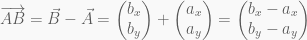
Vector Subtraction:
Suppose we have two points $\vec{A}$ and $\vec{B}$ and we want to find the displacement vector $\overrightarrow{AB}$ from a point $\vec{A}$ to point $\vec{B}$ . We can achieve this by simply subtracting the vector components of initial point $\vec{A}$ from the components of the terminal point $\vec{B}$ like so:

$\overrightarrow{AB} = \vec{B} - \vec{A} = \begin{pmatrix}b_x \\ b_y\end{pmatrix} + \begin{pmatrix}a_x \\ a_y\end{pmatrix} = \begin{pmatrix}b_x - a_x \\ b_y - a_y\end{pmatrix}$

From the picture we see that vector subtraction can be represented as a compound operation of both scalar multiplication and vector addition by negating the first vector (multiplying it by $-1$ ) and taking the sum of $-\vec{A}$ and $\vec{B}$ .

Magnitude:
Sometimes it is important to know how long a vector is along its direction. To do this we simply plug the vector components into the Pythagorean Theorem. I will use the notation $\|\vec{v}\|$ to represent the magnitude or length of a vector $\vec{v}$ with components $v_x$ and $v_y$ . So by the Pythagorean Theorem:

$\|\vec{v}\|^2 = v_x^2 + v_y^2 \implies \|\vec{v}\| = \sqrt{v_x^2 + v_y^2}$

The Pythagorean Theorem also works to find the magnitude of higher dimension vectors as well. For example, in three dimensions we have:

$\|\vec{v}\|^2 = v_x^2 + v_y^2 + v_z^2 \implies \|\vec{v}\| = \sqrt{v_x^2 + v_y^2 + v_z^2}$

This is useful because it gives us the absolute scalar distance between the vector’s initial and terminal point.

Normalization:
When we are dealing with directions, sometimes it is helpful to make sure that they have unit length (a magnitude of exactly one unit of measurement). Suppose we have a unit direction vector and a scalar velocity. To get the velocity as a vector we simply multiply the direction vector by the scalar velocity. But how do we get a normalized vector? Simple, we merely divide each of the vector components by its magnitude. I shall use the notation $\hat{v}$ to denote a normalized vector. So the formula for a normalized vector is simply:

$\hat{v} = \frac{\vec{v}}{\|\vec{v}\|} = \begin{pmatrix}v_x / \sqrt{v_x^2 + v_y^2} \\ v_y / \sqrt{v_x^2 + v_y^2}\end{pmatrix}$

Dot Product:
The dot product is one of the most useful operations in linear algebra and has many practical uses in making video games. It is often called the scalar product because it produces a numerical quantity. The dot product of two vectors $\vec{a}$ and $\vec{b}$ is defined algebraically for three dimensional vectors by the following formula:

$\vec{a} \bullet \vec{b} = a_x b_x + a_y b_y + a_z b_z$

Not very interesting at first, although it is worth mentioning that the dot product of a vector with itself is equivalent to the square of its magnitude. Also note that this property is not only commutative, but also distributive. That is:

$(\vec{a} + \vec{b}) \bullet \vec{c} = \vec{a} \bullet \vec{c} + \vec{b} \bullet \vec{c}$

However, where this formula draws meaning from is its geometric definition. Geometrically the dot product is defined as:

$\vec{a} \bullet \vec{b} = \|\vec{a}\| \|\vec{b}\| \cos{\theta}$

where $\theta$ is the minimum angle between the vectors $\vec{a}$ and $\vec{b}$ . The angle $\theta$ holds significant importance in a variety of situations from vector projection to collision detection. We can calculate the angle quite simply by rearranging the formula to get:

$\theta = \arccos(\frac{\vec{a} \bullet \vec{b}}{\|\vec{a}\| \|\vec{b}\|})$

If $\vec{a}$ and $\vec{b}$ are normalized vectors, this formula simplifies to:

$\theta = \arccos(\hat{a} \bullet \hat{b})$

However, there are many cases where it is not necessary to calculate the angle since the dot product is sufficient. This is convenient to programmers since the dot product is a much cheaper and more efficient operation than say the inverse cosine and anything that saves CPU cycles is a great boon to game programmers.

Cross Product:
The cross product is used in game logic in a variety of ways from game camera projection to quaternions. Since the cross product is most commonly used in terms of three dimensional space I will not cover how the cross product is applied to higher order vectors, despite the fact that their are applications for higher order cross products in game logic and computer graphics. Also keep in mind that all the vector operations covered thus far can be easily expanded to higher dimensions as well but are typically restricted to 2-4 dimensions (4 dimensional vectors are most commonly used in shaders to represent RGBA values).

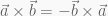
In general the cross product is a binary operation used to calculate a vector which is orthogonal to each of its input vectors. In the more practical terms of three dimensional space, it takes two vectors $\vec{a}$ and $\vec{b}$ and forms a third vector $\vec{c}$ which is perpendicular to both $\vec{a}$ and $\vec{b}$ and thus normal to the plane that contains $\vec{a}$ and $\vec{b}$ .

An important note to make is that the cross product of two vectors is NOT commutative. The order does matter in determining which direction the resulting vector points. In fact, the vector products $\vec{a} \times \vec{b}$ and $\vec{b} \times \vec{a}$ are related in the following way:

$\vec{a} \times \vec{b} = - \vec{b} \times \vec{a}$

So although they have equal magnitude they point in opposite directions. Additionally, how we actually calculate the cross product of two vectors depends on whether we are using left-handed or right-handed coordinates. It is important to understand this distinction because it depends on which computer graphics API you use as to which coordinate system you should use to write your cross product implementation. DirectX, for example, uses a left-handed coordinate system, whereas OpenGL uses a right-handed coordinate system.

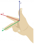
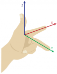
A right-handed coordinate system is simply a three dimensional coordinate system that satisfies the right-hand rule. The right-hand rule states that the orientation of the vectors’ cross product is determined by placing the x-axis and the y-axis tail-to-tail, flattening the right hand, extending it in the direction of the x-axis, and then curling the fingers in the direction that the angle the y-axis makes with the x-axis. The thumb then points in the direction of the z-axis. The left-hand rule simply follows the same procedure but with the left hand (See below).

The cross product in right-handed coordinates is defined as follows:

$\vec{a} \times \vec{b} = \begin{pmatrix} a_y b_z - a_z b_y \\ a_z b_x - a_x b_z \\ a_x b_y - a_y b_x \end{pmatrix}$ (right-handed)

In left-handed coordinates we get:

$\vec{a} \times \vec{b} = \begin{pmatrix} a_z b_y - a_y b_z \\ a_x b_z - a_z b_x \\ a_y b_x - a_x b_y \end{pmatrix}$ (left-handed)

Summary:

With this you should have a basic understanding of vector math and some of the ways it can be applied to video games. In my next post I will cover some more advanced things that can be accomplished with vectors along with some sample code written in C++. Click here for Part 2.

Resources:

Lay, David C. (2005). Linear Algebra and its Applications Third Updated Edition. Addison Wesley. ISBN 978-0-321-28713-4.

External Links:

Linear Algebra for Game Developers

Vector Math

What is Cripple Mr. Onion?

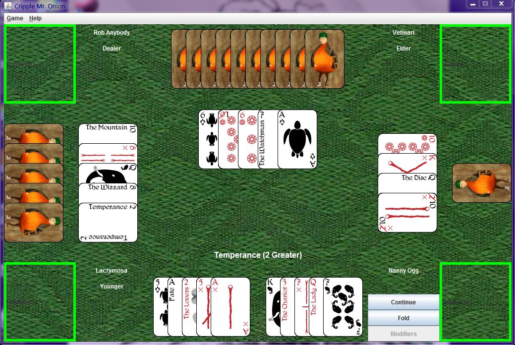
Cripple Mr. Onion was originally a gambling card game played by the characters in the fictional universe of the Discworld novels written by Terry Pratchett. Since no official rules have been set by the author himself, many Roundworld (our world) denizens have taken it upon themselves to create a set of rules for the game. One popular version was designed by Andrew C. Millard with help by Prof. Terry Tao and was even mentioned in the book Turtle Recall, which is a kind of Discworld encyclopedia written by Terry Pratchett himself. The book gives a vague description of the rules with the understanding that people playing the game are free to modify or ignore the rules as set. What follows is the unique interpretation I envisioned and I hope you will all enjoy playing it as much as I enjoyed creating it.

CMO Screen Capture Many versions of the game envisioned it with eight suits of cards much like combining two sets of regular playing cards but with the suits all different. The book Turtle Recall describes the deck as a regular set of playing cards combined with the complete Caroc deck (Discworld tarot deck). In my version there are a total of 78 playing cards divided up into six suits of thirteen cards each. The first four suits, turtles, elephants, staves and octograms are exactly like a regular set of 52 playing cards but with their suits renamed. The remaining two suits follow the same numbering scheme as the remaining four but have unique names for each card. The suits themselves are called the Lesser Arcana and the Greater Arcana and together they form the Caroc deck.

The game itself bears striking resemblance to both Poker and Blackjack. Like Poker there are various hand ranks that become exceedingly rare the higher their rank goes. Cards have number values just like in Blackjack and the rank of one’s hand is determined by how well you group the cards in your hand to sum to 21. However, what truly separates Cripple Mr. Onion from its Roundworld counterparts are the various optional rules that can be included. These are otherwise known as the “Modifiers.” A player may choose to use as many or as few modifiers as they wish with the exception of the Crippling Rule which is always active (hence the name Cripple Mr. Onion).

The user interface is built using Java’s swing library. The main application runs on the swing library’s Event Dispatch Thread (EDT). Meanwhile, the main game loop runs on the Engine Core thread and determines which animations need to be played and what the board should look like at various stages of the game. Whenever the core thread needs to start an animation, request input from the user or change the appearance of the board it calls a static method of the Application class to get an event object which it forwards to the EDT. This allows the core thread to make thread safe changes to the GUI.

The Application object loads all the necessary game resources and initializes the various swing components, some of which include a menu bar and glass pane as well as the content panes for various dialogs. The Application provides static methods for starting these dialogs with the appropriate modality and parent window. The menu bar provides the user with a list of game options and help tools which call these methods. The Table object represents the game view and acts as the content pane for the main window. It provides various public methods for changing the appearance of the board and for enabling and disabling certain components. The Animation Pane is the glass pane of the main window and is where all the animations are drawn.

Rendering animations using Swing components can be tricky since drawing only occurs when a paint event is dispatched by the EDT, a method known as passive rendering. The Animation objects in this game use threads that repeatedly update before calling the repaint method on the component to which they are attached. Then whenever a paint event is dispatched the given component’s paint method merely calls on the paint method of its attached Animation object.

// Animation.java

import java.awt.Component;
import java.awt.Graphics;
import java.util.ArrayList;

/**
 *
 * @author GK Potts
 */
public abstract class Animation implements Runnable {
    private final int SLEEP_DELAY = 25;

    protected ArrayList<AnimationListener> listeners;
    private Component context;
    private Thread currentThread;
    private long startTime;
    private long oldTime;
    private long currentTime;
    private boolean playing;
    private boolean running;

    public Animation() {
        listeners = new ArrayList<>();
        playing = false;
        running = false;
    }

    public abstract void paint(Graphics g);

    public abstract void update(long elapsed);

    ...

    @Override
    public void run() {
        long elapsed, sleep;
        running = true;
        currentThread = Thread.currentThread();
        startTime = System.currentTimeMillis();
        oldTime = startTime;
        for (AnimationListener listener : listeners) listener.onStart();
        while (running) {
            currentTime = System.currentTimeMillis();
            elapsed = currentTime - oldTime;
            if (playing) {
                update(elapsed);
                context.repaint();
            }

            oldTime = currentTime;
            sleep = SLEEP_DELAY - elapsed;
            if (sleep < 0) sleep = 2;

            try { Thread.sleep(sleep); }
            catch (InterruptedException e) { return; }
        }
    }
}

When an animation event occurs, an Animation object is constructed using position data collected from the Table. The Animation is then fitted with its own personal listener object whose methods are called whenever the animation is started, paused, stopped or reaches its end. The only one of these methods that is truly important is the OnComplete method because it notifies the core thread when the animation is finished. The Animation object is then attached to the Animation Pane and finally started on a new thread. Note that the animation thread does not need to be invoked on the EDT since it does not make any direct changes to the GUI. It merely calls the repaint method of the component to which it is attached. Repaint merely schedules a paint event to be executed later, thus making our Animations thread safe. If we ran our animation thread on the EDT our GUI would freeze until the animation thread ended.

In addition to having Animations for moving objects, this game also supports sprite based animations. Each time a card flips over or a modifier effect is activated, a sprite based Animation Clip object determines which frame to use based on the total elapsed time. This Animation Clip object is based almost entirely on the sprite based animation class that I wrote for use in the game engine I built for my previous game Captain Polly’s Booty. To see my blog posting on sprite animation click here.

The various Animation subclasses each utilize an Animation Data object which stores the position, rotation, and image data for each of the cards and provides helper methods for stepping forward the position, rotation and animation. Then using Hash Maps the animation objects map the Card objects to the Animation Data objects allowing the animation to simply cycle through the list of cards to update their positions and paint them. This way the order of the list determines what order to draw the cards in. Additional these data objects also store a rotated version of the image so that the program does not need to call the image rotation function, which is rather time consuming, within the paint method.

To prevent the clipping of images as a result of rotation each image is resized to a square whose sides are equal to the diameter of the circle that completely encloses the image. The images are then rotated about their center and position data is altered to take into account the change in size.

Player hands are evaluated through the use of two Objects: the Grouping, and the Hand Evaluator. Grouping merely looks at a set of cards and determines if it forms a valid card grouping and stores its overall ranking. Hand Evaluator looks at a player’s entire hand and attempts to create the best possible Grouping from the cards available. Hand Evaluator is also useful for evaluating possible hands by being able to generate modified copies of itself. These copies can then be compared to the original to see which one is a better hand.

Captain Polly’s Booty

Captain Polly’s Booty is a side-scrolling platform game originally based on the game Super Mario Bros. 3 for the NES. Super Mario Bros. 3 was the first video game I ever played and I have loved video games ever since. That is why for my college course on Game Programming I decided to create a platform game using one of my favorite sprites from Super Mario Bros. 3 as the model for my player character. Not weighted to the ground like in most games, the player is free to soar the skies as they guide Captain Polly in the search for his stolen loot.

The goal of the game is simple – to collect all of the crackers stolen from Captain Polly’s private collection. Though free to fly most places, the Captain must beware of strong winds that would push him into dangerous enemies and traps. Enemies may be disposed of with heavy objects dropped from above, but be careful because carrying heavy objects weighs him down. He must flap his wings even harder when laden, however being weighted down can sometimes be to his advantage.

Captain Polly’s Booty is written in C++ and uses Open GL and SDL libraries as well as standard C++ libraries. I built the game engine from scratch, but used the source documentation for the Unity3D Game Engine to model the objects and libraries that make up the core functionality of my engine. The application is single threaded and all the in-game logic is done within the main game loop.

At the start of each game loop the application stores the current input and time data into the static Input and Time objects so that it may be accessed by the behavior scripts attached to the various game objects. Then the game loop calls the Update functions of all the Game Objects and their Components. The next step is to update the physics portion of the game engine and to resolve any collisions that may have occurred due to a previous update. The physics runs on a different timeline than the rest of the updates and only updates if a specific amount of time has passed, but still runs on the same thread as the main game loop. Next the engine handles any events that have been added to the event queue. Lastly the engine draws the scene after sorting the various renderer objects according to their draw layer.

Many of the objects that I created for this engine are based closely on the Unity Engine. Some of these include the use of static Input and Time objects for retrieving up-to-date system information. Another element that I based off of Unity was the hierarchical relationship between Objects, Game Objects, and Components. I also put my math skills to the test when I created my own Math, Matrix, Vector, Transform, and Physics components and libraries. Among the other components that I have implemented are Behaviors, Animations, Colliders and Renderers.

While the Animation and Renderer objects are extremely stripped down for the sake of 2D drawing, the Colliders and Physics libraries should (theoretically) be easily expandable to apply to 3-dimensional space. Using support functions provided by the Collider objects, the Physics library uses the Gilbert Johnson Keerthi (GJK) collision detection algorithm as explained by Casey Muratori on mollyrocket.com. Click here to visit his blog. I also use the Expanding Polytope algorithm to determine collision depth and normal. For more on the mathematical concepts I used in my game engine please visit the following pages:

Game Programming: Math Libraries

Vectors Part 1: Introduction to Linear Algebra

Vectors Part 2: Programming in C++

Matrices and Transformations (Not yet available)

Quaternions (Not yet available)

Raycasting (Not yet available)

GJK Collision Detection (Not yet available)

Expanding Polytope (Not yet available)

Shapecasting (Not yet available)

A-Star Pathfinder (Unity)

During a team project for a college course on game engines, I worked on creating a game called Icebox Anchorage using the Unity3D game engine. During this time I built a pathfinding system that I intended to be used in our game. Sadly it never made it into the final version of the game because it turned out to be unnecessary. However, despite the fact that it was never utilized, it is still a fully functional system.

Using a set of nodes placed strategically about a scene, I formed a point-based grid that would act as the map that my pathfinding system would traverse. Then, using the A* search algorithm, enemy AIs would then have the ability to locate and chase the player even through winding corridors and mazes by locating a path to the node closest to the player. See a video demonstration below:

A* Algorithm:

The A* star algorithm is perhaps the most commonly used algorithm for finding the shortest path between two points on a map or grid. It is amalgamation of two other pathfinding algorithms: Dijkstra’s algorithm and Greedy Best-First-Search. Dijkstra’s algorithm works by procedurally visiting vertices in the graph in search of a shortest path. It maintains a two lists of vertices called the open set and the closed set. The closed set contains the list of vertices that have already been visited starting with only the starting vertex or node. As it does so it stores a value $g(n)$ representing the total distance traveled from the start node. Meanwhile, the open set contains all the vertices adjacent to those that have already been visited. Dijkstra’s algorithm works by repeatedly removing vertices from the open set starting with those that have the smallest $g(n)$ and adding them to the closed set until a path to the goal has been found or it has been determined that no such path exists. The problem with Dijkstra’s algorithm is that often most of the paths that it checks are useless making Dijkstra’s algorithm computationally expensive.

Greedy Best-First-Search works in a similar way in that it maintains an open and closed set of vertices. The difference is that instead of visiting the vertices closest to the starting point it visits the vertices closest to the goal vertex. This is calculated according to some estimate $h(n)$ called a heuristic. This is generally much more efficient than Dijkstra’s algorithm until it runs into an obstacle. Unfortunately, because it has to backtrack to find a way around obstacles, Greedy Best-First-Search often does not return a shortest path.

The A* algorithm takes the best of both these algorithms to find the shortest path in a way that ignores unlikely paths. For each vertex in the graph it keeps track of not only of the travel distance $g(n)$ to the node $n$ , but also that nodes heuristic value $h(n)$ . When choosing which vertices to visit first it goes by the vertices with the lowest cost value represented by $f(n) = g(n) + h(n)$ . This way it balances the two in a way that allows it to find a shortest path without being overly expensive.

Unity Implementation:

Two nodes are considered adjacent to one another if there is a straight line path between the two nodes. Each of the path nodes keeps a list of all the nodes that are adjacent to them. A separate GameObject called AI Map acts as the parent of all the path nodes in the level and contains the script that contains the A* algorithm. Here is how it was written:

public List<GameObject> FindPath(GameObject start, GameObject end) {
    // the set of tentative nodes to be evaluated
    Dictionary<GameObject, Node> open = new Dictionary<GameObject, Node>();

    // the set of nodes already evaluated
    Dictionary<GameObject, Node> closed = new Dictionary<GameObject, Node>();

    // map of the path taken to each of the node
    Dictionary<GameObject, Node> previous = new Dictionary<GameObject, Node>();

    Node startNode = new Node();  // g_value is given a default of infinity
    startNode.g_value = 0;
    startNode.f_value = Distance(start, end);
    open[start] = startNode;
    previous[start] = startNode;

    while (open.Count > 0) {
        // find the key value pair from the open set with the lowest f-score
        var current = open.Aggregate((a, b) =>
            (a.Value.f_value < b.Value.f_value)? a : b);

        // have we reached the goal?
        if (current.Key == end) {
            // reconstruct path and return;
            List<GameObject> path = new List<GameObject>();
            path.Add(end);

            Node scan = current.Value;
            // scan the list backwards
            while (scan  != null && scan.came_from != null) {
                path.Insert(0, scan.came_from);
                scan = previous[scan.came_from];
            }

            return path;
        }

        open.Remove(current.Key);
        closed[current.Key] = current.Value;

        PathNode node = current.Key.GetComponent<PathNode>();
        foreach (GameObject neighbor in node.adjacentNodes) {
            // ignore if the node has already been processed
            if (closed.ContainsKey(neighbor)) {
                continue;
            }

            // calculate the distance to the neighbor via the current node
            float tentative_g = current.Value.g_value + Distance(neighbor, current.Key);

            // Is this in the open set
            Node currentNeighbor;
            if (!open.TryGetValue(neighbor, out currentNeighbor)) {
                // if not create a new node with the maximum g-value
                // and add to the open set and map
                currentNeighbor = new Node();
                open[neighbor] = currentNeighbor;
                previous[neighbor] = currentNeighbor;
            }

            // Check if the new g-score is lower than the current one
            if (tentative_g < currentNeighbor.g_value) {
                // if so update the open set with this newly discovered shortest path
                currentNeighbor.came_from = current.Key;
                currentNeighbor.g_value = tentative_g;
                currentNeighbor.f_value = tentative_g + Distance(neighbor, end);
            }
        }
    }

    // no path found so return an empty list
    return new List<GameObject>();
}

The enemies contain a Seeker script that calls on the AI Map to find a path to its selected target. The target object as well as the points on the returned path require a SeekerTarget script. While the path nodes are considered to be static targets, the player is considered a moving target and in order to find a path to it, it is necessary to determine which path node it is closest to. Path nodes store direction vectors to each of their adjacent nodes as well as the midpoint between every pair of of nodes. This data is used to calculate the Voronoi region that each path node represents. Using the sign of the dot product of two vectors it is possible to determine which node the seeker target is closest to.