Most game engines define their own custom set of math libraries for use in their games. Unity, for example, has defined its own Mathf library for performing common operations on floating point numbers. You may wonder what is wrong with just using System.Math as apposed to UnityEngine.Mathf. Some people use Mathf instead of Math because it saves them the trouble of having to do double to float conversions. However, in most cases Math is considered faster than Mathf. Standard math libraries are certainly convenient and will most often be more efficient than any math libraries that you roll yourself, so why go to the trouble of implementing a custom library. The problem with standard math libraries is that they may not always have the kinds of functions that are most important to game programming. Other times it may be better to forgo accuracy in favor of efficiency by replacing expensive operations such as cos, sin and ex with less expensive and less accurate approximations of these functions. In this article I will discuss some of the most commonly used functions found in Unity’s Mathf library and how you may implement them yourself.
Approximately:
Due to the nature of floating point numbers it is very common for operations performed on them to result in some form of rounding error. This can lead to problems when trying to compare the equality of floating point numbers. For example we may end up comparing a number like 2.0 to a number like 1.999999999. For all effects and purposes these numbers are practically the same but when we check for equality we get a false statement. This is why we sometimes need to take into account some margin of error when comparing floats. This is exactly what the Mathf.Approximately function does. It can be implemented in the following way:
bool Approximately(float a, float b) {
    return Abs(a - b) < Epsilon;
}
Here we take the absolute value of the difference between the two input variables and check if it is less than some arbitrarily small value called Epsilon. It should be noted however that although some standard math already have a predefined value for epsilon, it may actually be better for the programmer to define their own value for epsilon since the standard math library’s definition of epsilon may be too small to make any difference from straight equality comparison. An alternative approach could also be to define an Approximately function that takes the tolerance as a parameter and just replace Epsilon with this tolerance value.
Clamp:
Clamp is such a useful tool that it is any wonder why it is not a common tool found in every math library, especially since it is so simple to write. Perhaps it is just so simple that some programmers feel it is not necessary to include it in a standard math library. Simply put, clamp ensures that its input value lies within a certain range of values. If the number lies between the given range it simply returns the number itself, otherwise it returns the nearest endpoint. An example where this might be useful is in the case where the programmer wants to ensure that a player character never goes past the edges of the screen. All the programmer has to do is Clamp the player’s position to within the screen boundaries. Clamp can be implemented in the following way:
float Clamp(float value, float min, float max) {
    return (value < min)? min : (value > max)? max : value;
}
This function is so useful that Unity has even included a Clamp01 function that specifically clamps a floating point value to between 0 and 1.
Linear Interpolation (Lerp):
Linear interpolation is the process by which we find a point somewhere between two input values. We can visualize it as a line drawn between two points. Using the equation for a line we can write the formula for the desired value 


![[0, 1]](https://s0.wp.com/latex.php?latex=%5B0%2C+1%5D&bg=f9f9f9&fg=555555&s=0&c=20201002)
![[a, b]](https://s0.wp.com/latex.php?latex=%5Ba%2C+b%5D&bg=f9f9f9&fg=555555&s=0&c=20201002)


float Lerp(float a, float b, float t) {
    t = Clamp01(t);
    return a * (1 - t) + b * t;
}
For more help learning the proper use of linear interpolation, see How to Lerp like a Pro by Robert Utter.
Move Towards:
While linear interpolation certainly has its uses, it is sometimes not entirely practical since it requires the programmer to know what point we started at and what fraction of the way between the two points we are at a given time. But suppose instead we want to procedurally step some value towards some target using some kind of displacement value. We want a way to find our new value while making sure that we do not overshoot our target. To do this we simply compare our expected displacement to the difference between our current value and our target value. If our expected displacement is greater than the actual distance to our target then we just return our target value. Here is an example:
float MoveTowards(float current, float target, float maxDelta) {
    float delta = target - current;
    return (maxDelta >= delta) ? target : current + maxDelta;
}
Note that in the implementation above a negative value of maxDelta will cause our output to procedurally step away from our target value.
Smooth Damp:
While MoveTowards generally serves its intended purpose it can often result in game mechanics that look somewhat jerky since it forces something to come to a sudden stop once it reaches its goal. If we want our game to look somewhat cleaner we need to apply smoothing to our calculations. One way that we can apply smoothing is to apply some kind of S-curve to give us that smooth ease-in/ease-out motion. One commonly used formula is 

Another technique to achieve smoothing is through exponential decay. This is a kind of ease-out method of smoothing and can be accomplished by the statement 

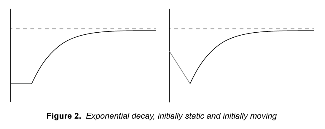
The approach we will be using, however, will rely on the model for a critically damped spring. This model fixes the problem we have with the exponential decay model by maintaining the ease-in property found in the S-curve.

A spring will always try to maintain a certain length by exerting a force that pushes it towards that desired length. Without damping this system will oscillate back and forth past the desired length forever. We say the system is critically damped when it returns to equilibrium in the least possible amount of time. We can write the equation for the force acted on the spring as 


The next step requires us to know how to solve for an equation of 


That was our particular solution; now let us find our complementary solution. The homogeneous DE gives us the characteristic equation 

It can be shown that the system will be critically damped when our equation has the real repeated roots 


In the above formula 


Solving for the constants 


This formula now tells us everything we need to calculate the new position and by taking the derivative we can find the new velocity of the object after after this time step:

Now the only parameters we need for our smoothing function are our current position and velocity, our target position our elapsed time and finally our smoothness factor 


One final note before we write our smoothing function is that Equation 3 and 4 contain 
float SmoothDamp(float current, float target, float& currentVelocity, float smoothTime,
        float maxSpeed = Infinity, float deltaTime = Time.deltaTime) {
    smoothTime = Max(0.0001f, smoothTime);
    float omega = 2.0f / smoothTime;
    float x = omega * deltaTime;
    float exp = 1.0f / (1.0f + x + 0.48 * x * x + 0.235 * x * x * x);
    float deltaX = target - current;
    float maxDelta = maxSpeed * smoothTime;

    // ensure we do not exceed our max speed
    deltaX = Clamp(deltaX, -maxDelta, maxDelta);
    float temp = (currentVelocity + omega * deltaX) * deltaTime;
    float result = current - deltaX + (deltaX + temp) * exp;
    currentVelocity = (currentVelocity - omega * temp) * exp;

    // ensure that we do not overshoot our target
    if (target - current > 0.0f == result > target) {
        result = target;
        currentVelocity = 0.0f;
    }
    return result;
}
Resources:
Kirmse, Andrew. (2004). Game Programming Gems 4. Charles River Media. ISBN 9781-58450-295-1.
Zill, Dennis G. (2009). A First Course in Differential Equations with Modeling Applications. Brooks Cole. ISBN 978-0-495-10824-5
External Links:
 and
and  we can visualize the first vector
  and
and  where
where  and its magnitude is called the scalar projection of
  . Similarly
 we can easily calculate
  where
where  is the angle between


 that we are reflecting and the normal
  of the surface that our vector is reflecting off. For simplicity we will assume that the normal vector is normalized.
 is the same as
  . Similarly, the projection of
  onto the plane whose normal is
  from
from 
 is quite simply a set, whose elements are vectors, for which we have defined two operations: vector addition and scalar multiplication. One example of
  . For the following operation we will be looking specifically at
  . A basis of a vector space is a subset of vectors
  in
in  for any scalar constant
  . We say that a basis spans a vector space so long as any vector
 . An orthonormal basis is simply a basis whose vectors are normalized and whose inner product is
  when
when 
 are an orthonormal basis representing the x, y and z coordinates of Cartesian space.
 . The only difference is that instead of scalar values we are using vectors for
  value to somewhere between
 and
and  are the initial position and velocity,
  is our target position,
  is the displacement vector,
 , and distributive, meaning that:
 and
and 

 . We see
 and
and  . Vector addition is both commutative and associative. Associative means that:
 .
. and
and  and we want to find the displacement vector
  from a point

 ) and taking the sum of
  and
and  to represent the magnitude or length of a vector
  and
and  . So by the Pythagorean Theorem:

 to denote a normalized vector. So the formula for a normalized vector is simply:


 and
and  are related in the following way:
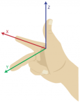
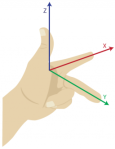
 (right-handed)
 (left-handed)